Data Preprocessing

09 Jan 2017

Aside

Data Preprocessing play a very essential role in the area of Knowledge Discovery. Usually the data in our live world is not whiten yet. The images are sometimes very noised i.g. by taken under improperly illumination conditions or the image itself is not clean etc.

Gaussian Filter

Gaussian filter enables us to remove the unnecessary information in images and retain the information that might important for representing the image. The basic idea is we just use some convolution operations with given kernel (ususally a matrix) to blur the small structure in images out, whereas the rough-textured blobs will be preserved. Usually the input image is a single channel gray image $\mathbf{S}_i = (s_i(x, y))$ . The pixel points $s_o(x, y)$ in output $\mathbf{S}_o$ is given by a convolution operation $\mathbf{K} = (h(u, v))$ with its neighbor point $s_i(x,y)$ . This operation is defined as follows:

$\begin{equation} s_o(x, y) = \frac{1}{m^2} \sum_{u=0}^{m-1} \sum_{v=0}^{m-1} s_i(x + k - u, y + k - v) \cdot h(u, v) \end{equation}$

where $m$ the filter size of the filter $\mathbf{K}$ and $k = \frac{m-1}{2}$ . Mostly it’s given by $m = 3, 5, 7, \dots$ .

Left: original image Right: the image after Gaussian filter

How much information will be blured depends closely on the size of filter. It’s a hyperparameter.

...
Mat tmp;
cv::GaussianBlur( img, tmp, cv::Size( 7, 7 ), 0 );
...

Digitalization

Some feature extraction needs binary image for extracting features such as histogram. So the original images should be digitalized, from which we got black and white points. Here we used Otsu method that clusters the pixels according to a threshold. The digitalized image looks like in figure below:

Left:original imageRight: the result after Otsu clustering

To get this image, we can use this function given by OpenCV

...
//thresholding to get a binary image
cv::threshold( tmp, tmp, 40, 255, THRESH_BINARY + CV_THRESH_OTSU );
...

Normalization

In our case the meters have various size. So the cropped images have also different size. The image ratio should be normalized without information lost, cause it also influence on the classification results.

Principle Component Analysis

Principle Component Analysis (PCA) is a widely used dimension reduction method in data preprocessing or data clustering area. The basic idea behind this algorithm is eigenvalue decomposition. We always search a direction, when the original data onto this direction or direction of a vector the variance of the projected data is maximized. In other words, the data is approximated as the data lying in this direction or space. If we have an unit vector $u$ and a data point $x$ , the length of the project of $x$ onto $u$ is $x^T u$ . Also this projection onto $u$ is also the distance $x^T u$ from origin. Therefore we maximize the variance of projection by choosing unit-length $u$ as in following Eq.:

$\begin{equation} \begin{split} \frac{1}{m} \sum_{i=1}^{m}(x_i^{T} u)^2 &= \frac{1}{m} \sum_{i=1}^{m} u^T x_i x_i^T u \\ &=u^T \left( \frac{1}{m} \sum_{i=1}^{m} x_ix_i^T \right) u, \end{split} \end{equation}$

the term in parentheses is actually the covariance matrix of original data. After solving this optimization problem we got the principle eigenvalue of covariance matrix $\Sigma = \frac{1}{m} \sum_{i=1}^{m} x_ix_i^T$ . We can project our data onto this eigenvalue vector $u_1, \dots, u_k, k < n$ , where $k$ and $n$ the dimension of eigenvector and original data. The projected data is calculated as follows:

$\begin{equation} y_i = \left[ \begin{array}{c} u_1^Tx_i \\ u_2^Tx_i \\ \vdots \\ u_k^Tx_i \end{array} \right] \in \mathbb{R}^k. \end{equation}$

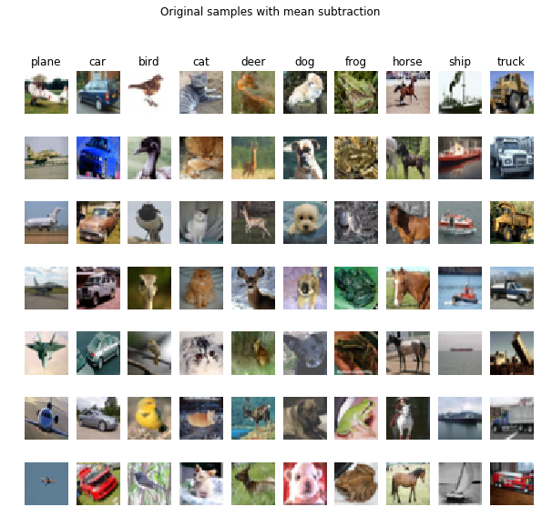
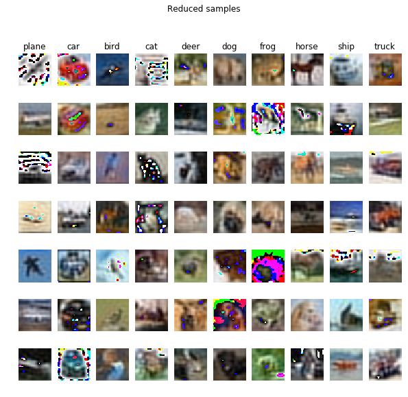
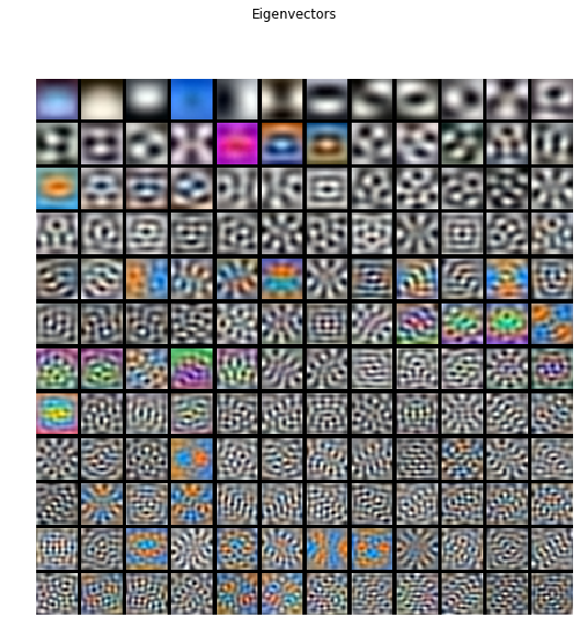
The mosttop image is normalized by subtracting the mean image. The image after dimension reduction is shown in middle.The bottom image shows the 144 eigenvalues.

Whiten

The only difference between PCA and Whitening is that the projected data is divided by the square root of eigenvalues. $\begin{equation} y_{w} = \frac{y_i}{\sqrt{\lambda_i}} \end{equation}$

Deep Convolutoin Neural Network