Feature Extraction
As in Introduction stated, the feature ensures the variablity of template in same classes to be minimized and maximized in different classes. We used the feature extraction approches that quite widely in image recognition.
Histogram
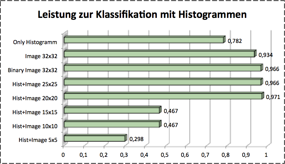
Histogram is a very simple method. It uses the frequency of a pixel color. Now we just have the binary image, which consist of black and white pixel. For getting a better classification I also put the original image as s extra information at the end of histogram features, cause sometimes the features are quite similar, for instance, the histograms of number 6 and 9 look quite same. The size of extra information should be optimized with cross validation approach. As validation result size in figure below we used 20x20 image as extra information to improve the accuracy. The histogram looks like:
Local Binary Patterns
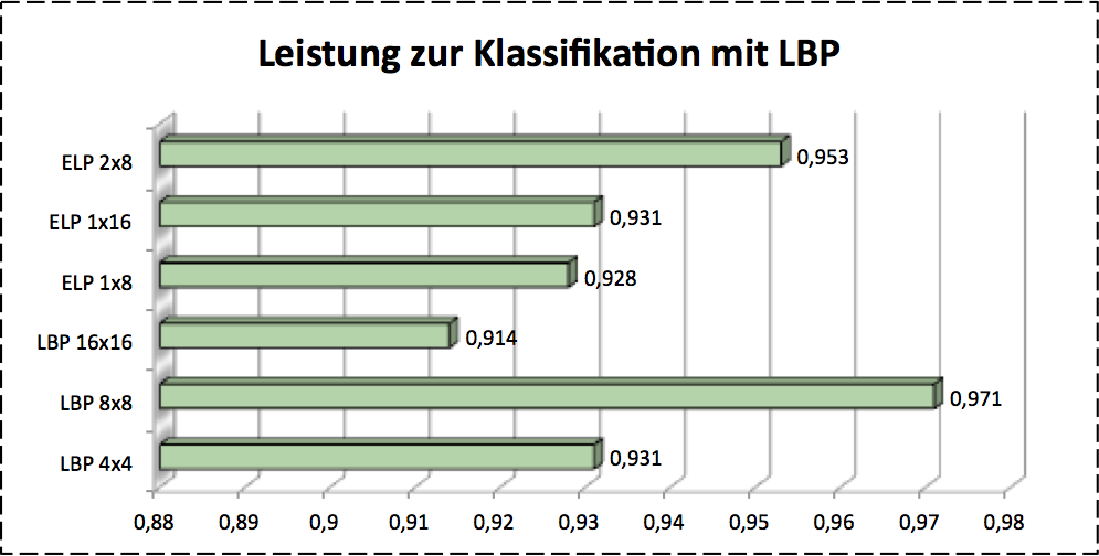
Local Binary Patterns (LBP) is based on the gray images. After a image splices in to small cells, it uses a very simple strategy to extract features. It picks eight neighbors of a pixel and compares the gray values at central pixel with his neighbors. Than we get a binary pattern. The frequency of this number is then as feature processed. Here the size of each cell is a hyperparameter of this operator. It should be cross validated.
Local Directional Patterns
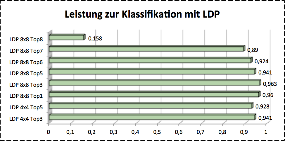
As the LBP is sensitive against noise, so I also had a look at the local directional pattern (LDP), which uses the kirsch mask to extract the top-K information that are important for a image. This kernel is defined as follows:
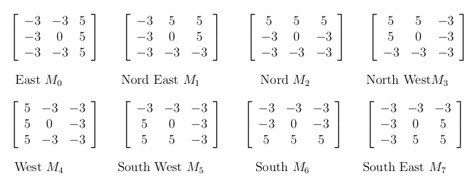
This kernels pays more attention for the basic form information i.e. the edges or the corner etc., because those objects are less sensitive against the illumination changes. Here we can select the top- components as our features. The size of should be investigated by cross validation.
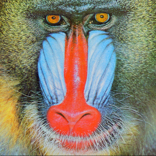
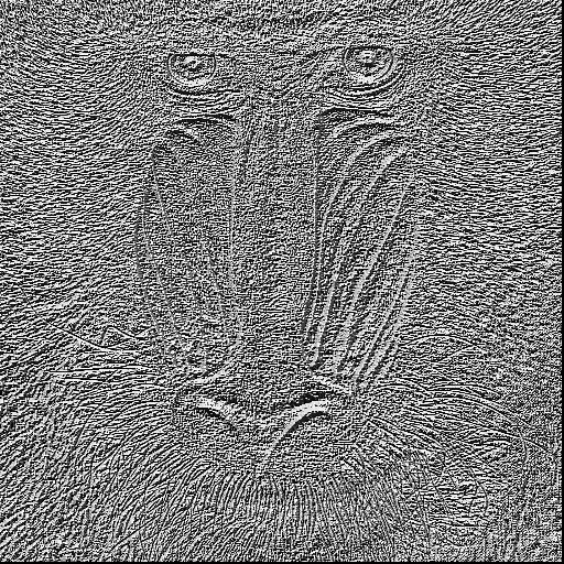
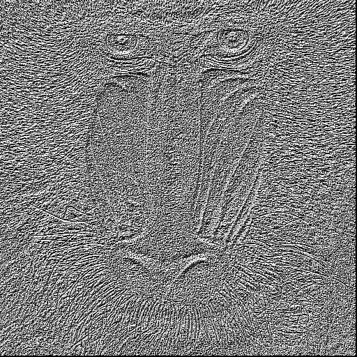
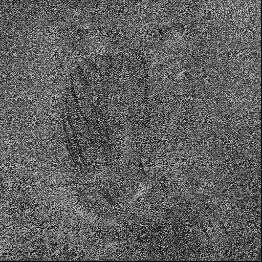
As we can see, the contour of baboon are found by different ways. Especially the one with Guassian noise, at this image the basic face pary has been slightly blured out, whereas the LDP only find the most relevant information with top-3.
Histogram of Oritend Gradient
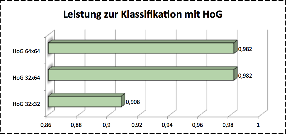
Histogram of Oritend Gradient (HoG) plays a critical role in object recognition, for it provides a good possibility to describing a object or its form as directional gradients. This feature looks like

To get this featuer we can use this function:
...
Mat hog = getHogDescriptor(img, descriptors, winSize);
...
The parameter winSize determins how big the image will be split into to calculate the HoG features.
Scale Invariant Feature Transform
Scale invariant feature transform (SIFT) is also a gray image based approach. We also used this operator, cause sometimes the number images are distorted by shaking the camera. As this points the scale invariant feature transform takes a scale invariant feature from images. This algorithm detects some feature that are not good for identifying the object. For instance the both circles at the bottom of image a) in figure below, although this sort of ability for catching the unnecessary characters is very helpful for template matching problem, which always spots the difference in images. Actually those poinst here detected are the results or difference of normalized Gaussian.

For accquiring the appropriate feature size we used corss validation. The image below shows the results.
Conclusion
SIFT works clearly worse in this case, so I don’t list it as compasion result. It’s shown clearly that HoG presents the best performance as so far. LDP shows different performance with different number of . It’s also imporved that the image plus histogram gives a good classification results.
After figuring out the best size of features for representing the original images, now we can feed this feature vectors as training data to training our classification models. It preceeds in following sections.