Model Candidate

15 Feb 2017

By now we got the training data. Which model is the best for our problem? We investigated the object recognition tasks such as street house number recognition, MNIST-benchdata classification and pedestrian detection etc. The models enjoy much privilege have been also considered in our problem.

Support Vector Machine

Support Vector Machine (SVM) presents a very easy understandable way for classification problems. The basis idea of it is derived from linear classifier. We want to find the support vectors that maximize the margin between two classes, which is depicted as follows:

Support Vectors and the optimal hyperplane

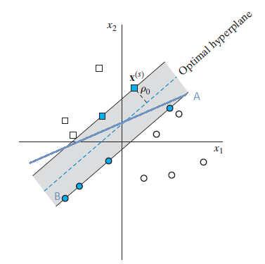
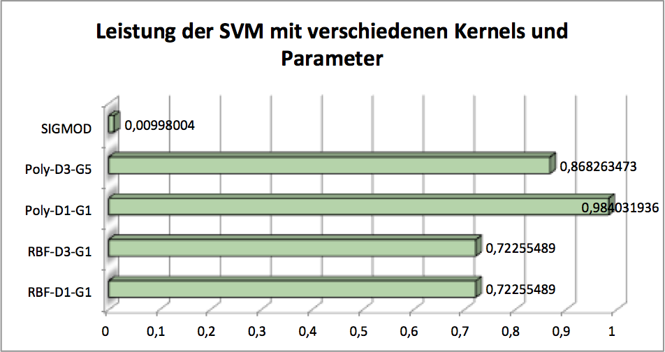
The dash line represents the optimal decision boudary between class $c_1$ and $c_2$, whereas solide line is just normal decision boundary that sepaerates them, but in a perfect way. Because our image class is a nonlinear classification problem, which means the data in input space is nonlinear separable. For solving this problem wen can map the data in input space into feature space, where the data is linear separable. The Kernel enable the mapping the data from input space to feature space, which is usually a doc product operation. Therefore sometimes kernel method is a alias of SVM. The ability of different kernels to classification varies, so we need to find out which the best kernel candidate for our problem. Ususally the polynomial kernel delieveries a good performance as in the other cases.

Multiple-layer Perceptron

Multiple layer perceptron (MLP) is inspired by the biological neural system. The network input function accept the input from the outside of the perceptron and continuously propagates the linear combination of inputs and their weights to the activation function. The classification will be then executed according to the comparing the activation function’s output with an threshold values. For solving the nonlinear classification problem we built multiple layer perceptrons, whereby the neural perceptrons in input layers read the data. Than activation process are aroused in each perceptron. The neural perceptron in different layers are connected synapticly and not connected in the same layers.

The net works generally in two phases: Forward propagation:, in which the function signals are propagated forwards from layer to layer till it reach the output layers. In output layer we usually get a score for each class. According to this scores we just send the adjustment message backwards layer to later, which is the Backward propagation, in this process the parameters will be adjusted according to the classification scores. This is actually sometimes called blame assignment problem. It means how the errors will be assigned to where it probably aroused potentially. The structure of the nets or the parameters such as the weights of neurons, the number of hidden layers are very important for the final classification results. Theses parameters should be investigated by validation. As the validation resuts show in the figure,

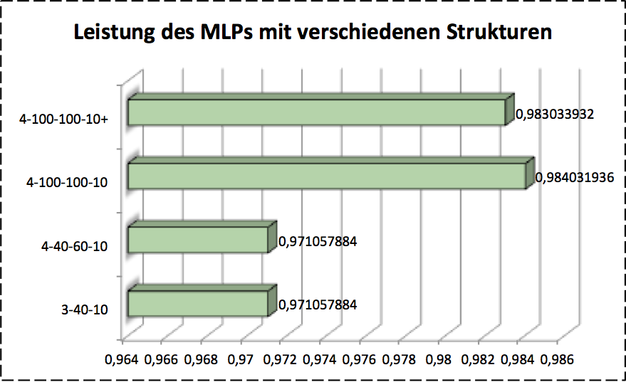
the number of neurons in hidden layers play a role for final classification accuracy. Descripe all complicated models, normally the 3 layers MLP (without counting input layers) is the best structure for classification problem.

k-Nearest Neighbor

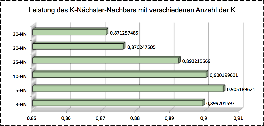
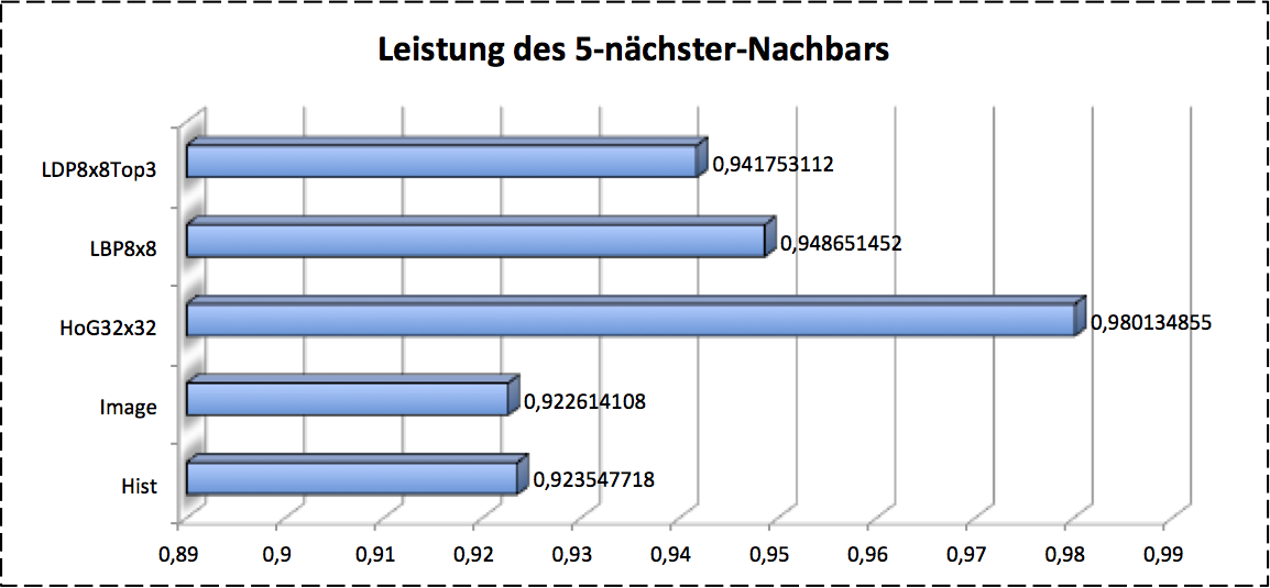
$k$-Nearest Neighbor KNN is a lazying methods. What we need for this method is just a hyperparamter of $k$ and a labeled dataset. When a test object comes, this algorithm calculates the similarity of this object between all training objects by using some distance measure approaches such as euclidean distance. As said before, this algorithm requires a large memory resource on demand for loading the all training data, that’s why it’s called lazying learning method. Further more it takes much longer time than other models during prediction or classification. By comparing the similarity between test object and all training data we’ll get a dataset, which is the $k$-nearest neighbor of test object. The final label of test object is the most frequent labels in this dataset. After validation we got the $5-$ nearest neighbor brings the best accuracy for our problem as shows as follows:

As you can see either SVM, MLP or KNN works individually. Is it possible that we can combine the basic single model together to get a better performance? By using this idea we can boost the basic models or adaboost a single model many times.

Boosting

Boosting consists of so-called basic classifiers usually. The final result of this model will be voted by these basic classifiers. It works as follows: we used the three models we introduce before as basic classifiers. Here we go! The training data is split into three training datasets $t_1, t_2, t_3$. The first basic model $m_1$ will be trained on $t_1$ at first. Then the trained $m_1$ is used for predicting the dataset $t_2$. The incorrectly classified training data with the same size of training data in $t_2$ will be used for training $m_2$. After it the dataset $t_3$ will as test data for $m_1$ and $m_2$ predicted. The misclassified data will be then used for $m_3$. For Boosting we used SVM, MLP, $k$-NN as basic classifiers. The boosted results show as follows:

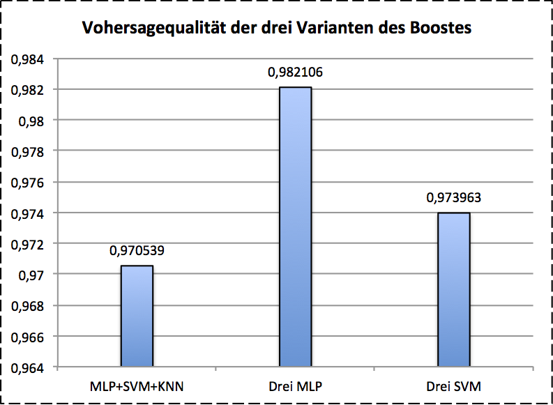
The boosted MLP gives the best performance on validation data.

AdaBoost

AdaBoost uses a hyperparameter of number of basic classifier and the selected basic modal, i.e. we trained before. Our concepts is based on Multi-class AdaBoost and works as follows: this algorithm pays more attention for the misclassified samples during the training process. Each training sample has a initialized weight at the beginning of training and each basic model also has a confidence weight. As the model trains, the misclassification error will be calculated as well as the error of basic model. The weight of training samples is also updated by using the confidence weight of classifiers. The weight should be normalized after each updating. The label of test object of this model will be given according to the confidence of basic models af last.

For AdaBoost I used the 3 MLP (plus HoG) as basic model. The boosted result is shown as in following figure.

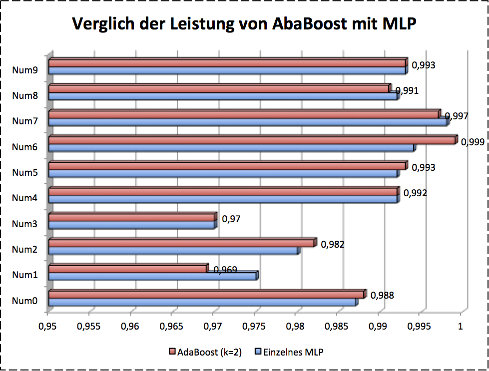
Some of numbers are clearly improved by AdaBoost and some are not good enough.

Conclusion

As we investigated, different features and models give us various classification performance. The next step is to combine all of them to find the best combo-candidate as our final classifier. The results are given as follows:

Top: polynomial kernel with different feature extractions Middle: mlp with different feature extractions Botton: 5-NN with different feature extractions

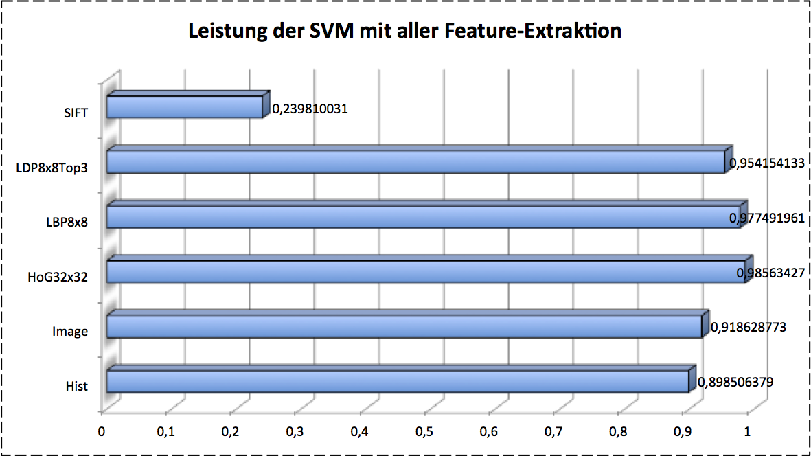
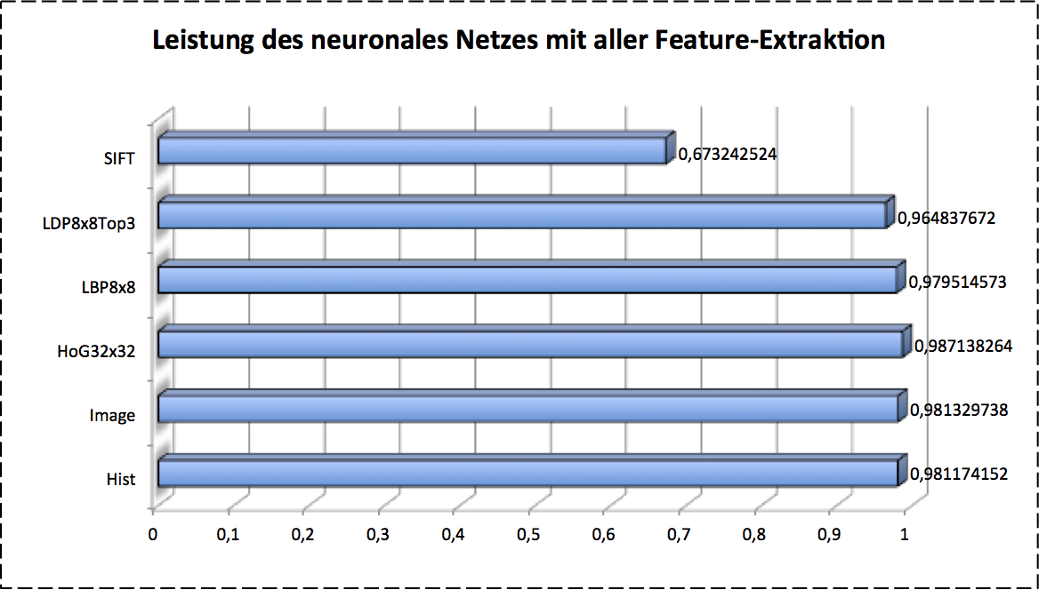
As so far we introduced the classical pipeline of image recognition with machine learning. It looks canonically and works well in previous decades. The most critical point of final performance to classifying is the feature extraction, if we only consider the classification model is given in advance. In other words, it accquires very intensive expert knowledge on image processing. This should be reconsidered in feature.