Long Short Term Memory

02 Jun 2017

Introduction

Long Short Term Memory (LSTM) differentiates with RNN only by holding a cell state in each time step. Furthermore the hidden state will be split in four single cell states. These cell states have the ability to add or remove information during time steps, which are organized by special non-linear structures called gates. Let’ walk it though out.

The working flow in LSTM

The evolution of LSTM over time steps is shown as follows:

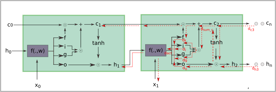
The $f(.,w)$ is an affine operation that calculates the activation vectors. As it depicts here, the activation signals have been split into four slices: input gate $i$ , forget gate $f$ , output gate $o$ and go through gate $g$ . The $i, f, o$ gates are kind of sigmoid functions that maps its inputs to interval $[0, 1]$ and go through gate uses $\tanh(.)$ to squashes its inputs to interval $[-1, 1]$ so that the output looks more centralized.

Forward phase

In forward propagation phase the input gate $i$ decides what we want to process and go through gate $g$ determines how much signal we want to let it through. The forget gate $f$ gives signals (here previous cell state $c_0$ ) the possibility that it always has been taken into account in next cell state $c_1$ . The squashed new state $c_1$ is merged with output gate $o$ ’s outputs for generating new hidden state $h_1$ .

This forward process can be abstracted as the following equations:

$\begin{equation} \begin{split} h_n &= o_{n-1} \odot \tanh(c_n) \\ &= o_{n-1} \odot \tanh(f_{n-1} \odot c_{n-1}) + i_{n-1} \odot g_{n-1}, \\ \end{split} \end{equation}$

where $\odot$ is element-wise product and the gates are just subslices of activation vectors like $o_{n-1} = sigmoid(act[:,2,:])$ and $g_{n-1} = \tanh(act[:,3,:])$ etc. $n$ denotes the time step. The act here means the activation vectors we got from the $f(.w)$ function. As forward propagation starts, the initial cell state $c_0$ is initialized as same size of hidden state $h_0$ then all the time evolutions work out iteratively through. Here we also used $L2$ -Norm as regularization penalty like we always do in neural networks.

Backward phase

In Backward propagatoin phase, the gradients of cell state and hidden state are back propagated in the symmetrical order that got forward propagated. Assume we have the derivate of $c_3$ and $h_3$ as $d_{c3}$ and $d_{h3}$ , now let’s back propagate the errors. Keep in mind that what you calculated in forward propagation should be cached for back propagation and all gradient-flows has exact the invertible direction of forward propagation. Taken $d_{h3}$ and next cell state $c_3$ we got the gradient of previous output gate as follows:

$\begin{equation} \begin{split} d_{o_2} &= d_{h3} \times \tanh(c_3) \times \nabla_{sigmoid(o_2)},\\ &= \underbrace{d_{h3} \times \tanh(c_3)}_{derivate\ of\ h_3\ backward} \underbrace{\times}_{distributes\ the\ gradients} \underbrace{o_2 \times ( 1 - o_2),}_{numerical\ derivative\ of\ sigmoid\ for\ output gate}\\ \end{split} \end{equation}$

from which we got $o_2$ in the diagram above. Be careful that we did not use $d_{c3}$ for gradient of $o_2$ cause that does not contribute to calculate the $c_3$ . In contrast to this the gradient of next hidden state $d_{h3}$ is a little bit complicated to back propagate. For getting $h_3$ we used $c_2$ and $o_2$ , $c_2$ is derived from $c_1, f, i, g$ , here takes more attention. $d_{sum_c}$ in above figure coalesces the two flows from cell state $d_{c3}$ and $d_{h3}$ , it’s merged as follows:

$\begin{equation} \begin{split} d_{sum_c} &= d_{h3} \times o_2 \times \nabla_{\tanh(c_3)} + d_{c3} \\ &= d_{h3} \times o_2 \times (1 - \tanh(c_3)^2) + d_{c3}, \\ \end{split} \end{equation}$

after this the gradient flow will be back propagated to $f, i, g$ continuously. The derivate of forget gate $f_2$ calculated as:

$\begin{equation} \begin{split} d_{f2} &= d_{sum_c} \times \nabla_{sigmoid(f_2)} \times c_1 \\ &= d_{sum_c} \times f_2 \times ( 1 - f_2) \times c_1. \\ \end{split} \end{equation}$

In the same way we got derivate of $i_2, g_2$ separately as follow:

$\begin{equation} d_{i2} = d_{sum_c} \times i_2 \times ( 1 - i_2) \times g_2, \\ \end{equation}$ $\begin{equation} d_{g2} = d_{sum_c} \times ( 1 - g_2^2) \times i_2. \\ \end{equation}$

As so far we can concatenate all the gate derivatives for assembling the derivate of activation vectors, from which we’ll get the derivative of hidden state’s weight, input to hidden state’s weight as well as the derivate of initial cell state and bias, which is just a couple of matrix multiplication and will not be further explained here.

For overfitting a model we used the same setting as in RNN, the loss of LSTM changes very mildly than RNN. Although the captioning results of both models are nearly same, but the LSTM has an advantage for again Vanishing-gradient problem.

Conclusion