Tensorflow
Tensorflow (TF) is open-source library for numerical computation for machine intelligence. It’s developed by Google and used for working on Google Brain project. TF has also some speciality. It uses the computational graph to build scalable models to one or more CPUs and GPUs. All the operations are represented as nodes in computational graph and the data containers such as tensor, matrix, vector are assigned to the edge of this graph. Formally to say the graph embodies the necessary parts for computations.
Syntax
All the nodes and edges only has computational mean when it run in a session that encapsulates the running time of a computational model. It has different variable types. The basic type i.e. constant that holds a constant in nodes. For instance we initialized a constant variable in TF is defined as follows.
...
# Import Tensorflow
import tensorflow as tf

# Constant node in graph
c = tf.constant(3.0, tf.float32)

# Variable will get values later
a = tf.placeholder(tf.float32, shape=[None, 10])
b = tf.placeholder(tf.float32, shape=[None, 10])

# Operator in graph
add_node = a + b

# Trainable variable with initial value and data type
W = tf.Variable([.3], tf.float32)

# Runtime encapsulator for TF
session = tf.Session()

# Initial all variables
init = tf.global_variables_initializer()
session.run(init)
...
Another variable is that means the value of this variable will be assigned later liked we defined . The addition operator defined just like in normal computer language. The makes this variable learnable. As a session initialized, then we can invoke its run function to launch our computation.
Working on TF
After a brief syntax introduction in TF we’d like use it to experience how it work in image classification on CIFAR-10 data. The process is quite easy, for simplicity you can use to build your computational graph, but I’d like to build it more natively. The follows structure will be used in our model:
- 7x7 convolutional layer with 32 filters and stride of 1
- ReLU activation layer
- spatial batch normalization Layer (trainable parameters, with scale and centering)
- 2x2 max pooling layer with a stride of 2
- affine layer with 1024 output units
- ReLU activation layer
- affine layer from 1024 input units to 10 outputs.
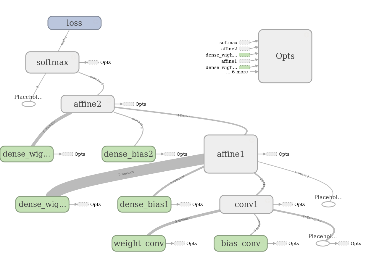
The inputs will be convoluted with convolution layer, so we need both weight and bias for this layer. As the input images have three channels () , so the weight tensor in TF is organized as [7, 7, 3, 32], each filter has a bias parameter. The output of convolution layer can be either in batch normalization or ReLU layer fed. After it the output in ReLU will be max sub-pooled in size 2x2 with a stride of 2. The output of sub-pooling layer will be fully connected with a feed forward neuron layer. With ReLU it will activated and be connected in the output layer with 10 neuron. This computation graph in the following figure. It explains clearly how the graph connected and how the data flows.
This graph can be built in the following code piece:
...
#7x7 Convolutional Layer with 32 filters and stride of 1
with tf.name_scope('conv1'):
  with tf.name_scope('weight'):
    WC1 = tf.get_variable("weight_conv", shape=[7, 7, 3, 32])
    variable_summaries(WC1)

with tf.name_scope('bias'):
  bc1 = tf.get_variable("bias_conv", shape=[32])
  variable_summaries(bc1)

# Convoluton layer
with tf.name_scope('conv2d'):
  h_conv1 = tf.nn.conv2d(X, WC1, strides=[1,2,2,1], padding='VALID') + bc1
  print ("h_conv1.shape",h_conv1.shape)

# Batch normalization layer
#with tf.name_scope('batch_norm'):
#    batched = batch_normalization(h_conv1, 32, is_training, 'batch_norm')

# ReLU activation nayer
with tf.name_scope('ReLU'):
  #h1_relu = tf.nn.relu(h_conv1)
  h1_relu = tf.nn.relu(h_conv1)
  print ("h1_relu.shape",h1_relu.shape)

# 2x2 Max Pooling layer with a stride of 2
with tf.name_scope('pooling'):
  h_pool1 = max_pool_2x2(h1_relu)
  print ("h_pool1.shape",h_pool1.shape)

with tf.name_scope('flatten'):
  h_pool1_flat, channels = conv2d_flatten(h_pool1)
  print ("h_pool1_flat.shape",h_pool1_flat.shape)

with tf.name_scope('affine1'):

  #with tf.name_scope('batch_norm'):
  #    batched = tf.nn.batch_normalization(h_pool1, 0, 1, )

  # Affine layer with 1024 output units
  with tf.name_scope('weight'):
    WFC1 = tf.get_variable("dense_wight1", shape=[channels, 1024])
    variable_summaries(WFC1)

  with tf.name_scope('bias'):
    bfc1 = tf.get_variable("dense_bias1", shape=[1024])
    variable_summaries(bfc1)

  with tf.name_scope('output'):
    output = tf.matmul(h_pool1_flat, WFC1) + bfc1

  with tf.name_scope('batch_norm'):
    batched = batch_normalization(output, 1024, is_training, 'batch_norm')

  # ReLU Activation Layer
  with tf.name_scope('ReLU'):
    h_fc1 = tf.nn.relu(batched)
    variable_summaries(h_fc1)
    print ("h_fc1.shape",h_fc1.shape)

with tf.name_scope('affine2'):
  # Affine layer from 1024 input units to 10 outputs
  with tf.name_scope('weight'):
  WFC2 = tf.get_variable("dense_wight2", shape=[1024, 10])
  variable_summaries(WFC2)

with tf.name_scope('bias'):
  bfc2 = tf.get_variable("dense_bias2", shape=[10])
  variable_summaries(bfc2)

with tf.name_scope('output'):
  y_out = tf.matmul(h_fc1,WFC2) + bfc2
  tf.summary.histogram('activations', y_out)
...
After convolution the activated featuers are as inputs in dense neural layer applied. The output of this dense layer is connected to the output layer. The whole graph will be launched with calling .
Softmax
The softmax in output layer is calculated as follows:
# define our loss
with tf.name_scope('softmax'):
    total_loss = tf.losses.softmax_cross_entropy(tf.one_hot(y,10),logits=y_out)
    tf.summary.scalar('cross_entropy', total_loss)
with tf.name_scope('loss'):
    mean_loss = tf.reduce_mean(total_loss)
    tf.summary.scalar('mean_loss', mean_loss)
needs the output in our graph, and is the ground truth.
Optimizer
Compared with optimizer we used before, in TF it involves just a API call. At first get the update collections, then you assign the optimizer you use, the learning rate for optimizer and what you want to minimize, here we intend to minimize the mean_loss we calculated before.
with tf.name_scope('Opts'):
    extra_update_ops = tf.get_collection(tf.GraphKeys.UPDATE_OPS)

    with tf.control_dependencies(extra_update_ops):
        train_step = tf.train.AdamOptimizer(1e-4).minimize(mean_loss)
Visualize Graph
With TensorBoard you can check your computaional graph that we built before. To achieve this you should do a little more works as usual, but it’s also quite simple. Before you seesion is launched, you should assign the log path to save your computational logs.
...
log_path_train = 'VisualBoard/train'
log_path_test = 'VisualBoard/test'
...
Those two lines create two folders named train and test separately in directory VisualBoard. TensorBoard will parse the log your graph generated and summaries it to build the graph you want to check. After running the code to build graph, it still does n’t exist untill you call the API.
with tf.Session() as sess:
    # Tensorflow will gather all the summary information for visualization later
    merged = tf.summary.merge_all()

    # Where the train/test log goes to
    train_writer = tf.summary.FileWriter(log_path_train, sess.graph)
    test_writer = tf.summary.FileWriter(log_path_test)

    # Using GPU or CPU to run session "/cpu:0" or "/gpu:0"
    with tf.device("/gpu:0"):
        # Initialize all the global variables firstly
        sess.run(tf.global_variables_initializer())

        # run you graph in minibatch model
        run_model(sess,y_out,X_train,y_train,10,64,100,train_step,True)
Just one last step to visualize the graph. After running you model out, you should invoke the visualization command to build the image we saw before. Using the following command in terminal window
tensorboard --logdir=VisualBoard/trainHere we go, you will get a windows like this:
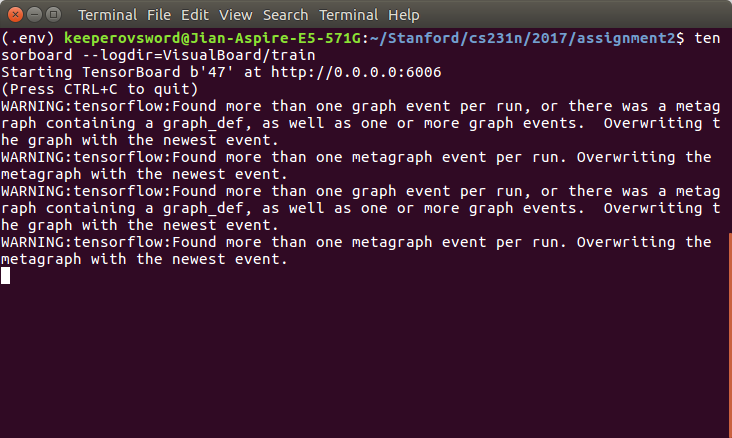
Just click the http addres you will see the graph we saw before.
Conclusion
As you can see, building a deep learning model in Tensorflow is quite consice. What you need is define the forward propagation. After it, you can kick-off the run time of compuation session to let you compuataional graph comes alive. You can pull the whole project and have a try with TF! Have fun with that!