Eligibility Traces

07 Jun 2017

Aside

As so far, either Model-based Methods or Model-Free method enables us the find the optimal policy, but not effectively. In this section we’ll use some extra information to make this process much easier.

Eligibility Traces

What’s eligibility traces? To answer this question, we can glance the two different views of eligibility traces. From mechanistic view, be short, it’s a extra tracing information with that the learner learns much more effectively than the general methods, this mechanistic view is also noted as backward view, depicted in the following figure.

The mechanistic view of eligibility traces

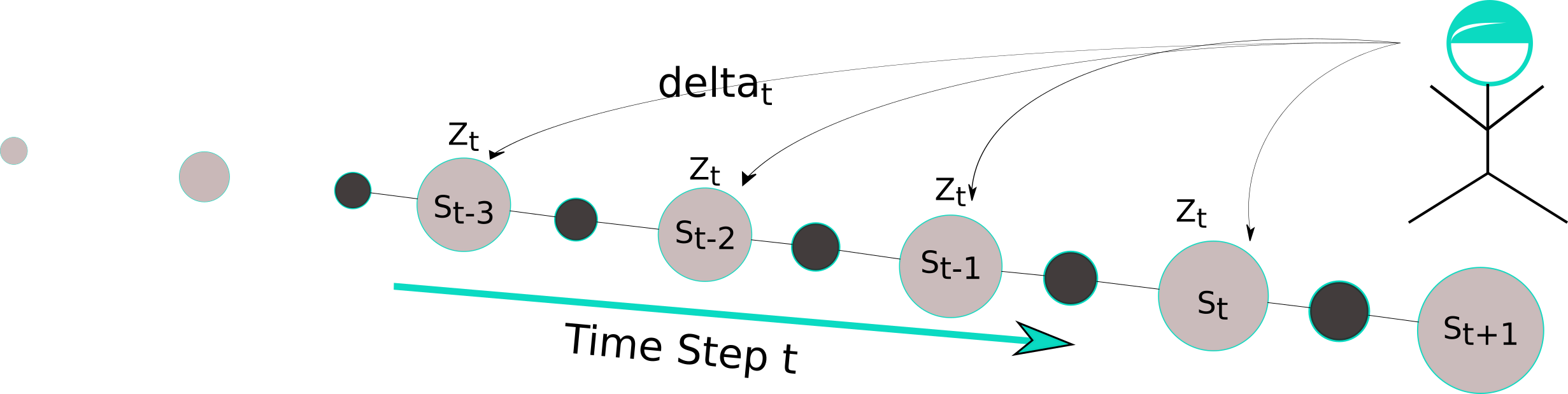
For holding this eligibility traces we need a extra memory variable for each state. In a episode we take an action $a$ under the current $\pi$ for state $s$ and we get a reward $R$ and next state $s^\prime$. The temporal difference is given by

Meanwhile the counter of state be accessed will be updated. After it all the state value of each state will be updated with considering the $\delta$ and eligibility variable will be also discounted by the discount factor and eligibility factor $\lambda$. Once the agent reaches a terminal state or a state with high reward, then this information will be back propagated towards to all the state in terms of the $\lambda$ eligibility trace. Almost every TD-method can be combined with eligibility trace to work better. The another view is the theoretic view, also as forward view noted and depicted in Figure:

The theoretic view of eligibility traces.

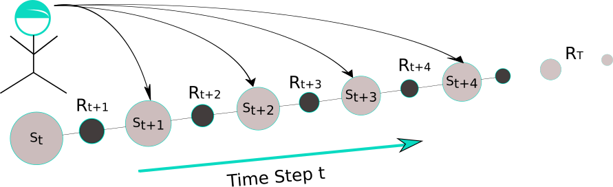
It’s a bridge between TD-Learning and MC-method. It updates the current state by looking ahead and taking the future states into account. When just only time step is considered, then it turns not surprisingly out that it’s the 1-step TD-method likes $v_\pi(S_t)^{(1)} = R_{t+1} + \gamma V(S_{t+1})$, whereas the MC-methods performs a backup for estimating state value for each state based on the entire sequence of observed rewards from that state until the end of this episode, formally it looks like in \begin{equation} v_\pi(S_t) = R_{t+1} + \gamma R_{t+2} + \gamma^2 R_{t+3} + \dots + \gamma^{T-t-1}R_T. \end{equation}

for which we have the sequence events $S_t, R_{t+1}, S_{t+1}, R_{t+2}, \dots. R_T$ and $T$ is the last time step in this episode. Make this equality more generally, we have the “corrected $n-$step truncated return”: \begin{equation} v_\pi(S_t)^{(n)} = R_{t+1} + \gamma R_{t+2} + \gamma^2 R_{t+3} + \dots + \gamma^{n-1}R_{t+n} +\gamma^n V(S_{t+n}). \end{equation} It means the current state is truncated after $n-$steps and corrected by adding the estimating value of $n-$th next state. In this point of view we can solve either continuous or episodic tasks as well. MC-method is just special case that $T-t <n$. I used the $Q(\lambda)$ to solve the four-gates problems. As this approach beings, it works exactly likes the Q-learning. Once the agent gets the terminal state, the situation changes. This trace information has been used in next iteration repeatedly and enables the algorithm to get converge much quickly.

Dyna-Q is an another TD-learning method that also builds the transition model of environment during the learning. It integrates the planning and control as whole one part. At first the agent tries to learn and to find the optimal policy just like Q-learning does. Meanwhile the model of the environment will be calculated. Then this model will be used to update value state of all states. Sometimes it works well, if the model is optimistic. But if the environment is stochastic, the performance of this method will be downgraded by the uncertainty of environment, in other words, by the wrong estimated model. For this problem we can reconsider the trade-off between exploration and exploitation and some heuristic strategies.