Model-based Method

07 Jun 2017

As mentioned in Shortest Path previously, we want to find a optimal policy, so our agent can get much more rewards and few penalty. This policy is acquired by the interaction of the agent with environment. As the agent works, we should use the feedbacks to extract the policy informations as we can. For it we need a mechanism to describes how a state good or bad for the agent is. In other words, what penalty informations exist at states in environment. This policy is given described by the value function accordingly. Let’s clarify the definition of policy. A policy is mapping from each state $s \in S$, and action $a \in A$, to the probability $\pi(s,a)$ of taking action $a$ in state $s$. So the value function of a state $s$ under a policy $\pi$ denoted as $v_{\pi(s)}$ is a expected return when agent starts from $s$ and follows the policy $\pi$ over times. In MDPs the value state function for policy $\pi$ is defined as

The Optimal policy is defined as: $v_\star(s)= \sum_{a} \pi(a|s) \sum_{s^\prime}p(s^\prime|s,a) \left[ r(s, a, s^\prime) + \gamma v_\pi(s^\prime) \right]$,

where $G_t$ is the return in $s_t$ and $\gamma$ the discount rate, which means how much contribute of the future state will be considered in calculating the current state value. This is equation is so-called $\color{red}{Bellman\ Equation}$. It reflects the relation between the value of state and its successor state. For iterations we can use back-up to make it easier to understand. The Backup for $v_\pi$ and $q_\pi$ is represented as:

Back-up diagram at states

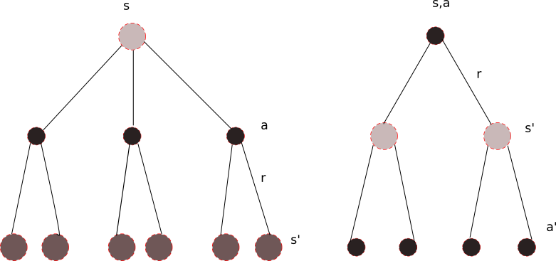
The solid circles mean the state-action pair and empty circles mean state. What Bellman Operator shows us is that the value in state $s$ is the weighted sum (the second sum operator in equation) of all successor state by the probability of occurring (the first sum operator).
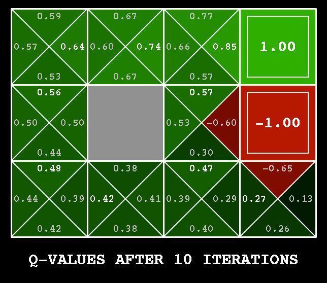
Correspondingly the Q-value of a state $s$ taking an action $a$ under policy $\pi$ is defined as: $q_\pi(s,a) = \mathbb{E}\left[ G_t|S_t = s, A_t = a \right]$ $= \mathbb{E}_\pi \left[ \sum_{k=0}^{\infty} \gamma^k R_{t+k+1}|S_t = s, A_t = a \right]$

$q_\star(s,a) = \sum_{s^\prime}p(s^\prime|s, a) \left[ r(s,a,s^\prime) + \gamma \max_{a^\prime}q_\star(s^\prime, a^\prime) \right],$ which is called action value function for policy $\pi$.

The goal is to finding the optimal policy that the corresponding function can be maximized greedily. Once the optimal value function is determined, it’s easy to get optimal policy.

As so far we give an explanation why do we need value function or action value function, in following section I’ll show some concrete algorithms for investigating the optimal policy. All of them share the same property: they are all tabular methods. It means all the state values are stored temporally in tabular data structure.

Policy Iteration

Policy Iteration (PI) is dynamic programming operator, it’s shown in the following Fig.

Policy Iteration

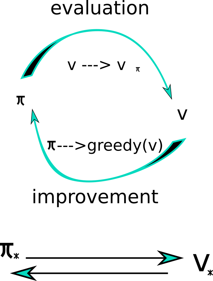
The given policy will be at first evaluated in a very simple way: for $s \in \mathcal{S}$, the current state value is backed up. In current state $s$ its new state value function
$v(s)\leftarrow \sum_{s^\prime}p(s^\prime|s,\pi(s)) \left[ r(s, \pi(s), s^\pi) + \gamma v(s^\prime) \right]$

will be iteratively calculated. After it the difference of two function value at current state $s$ will be compared with some given accuracy parameters till it converges. In policy improvement we select the action that maximizes the current state value like $\pi(s) \leftarrow \underset{a}{\operatorname{argmax}} \sum_{s^\prime} p(s^\prime|s,a) \left[ r(s, a,s^\prime) + \gamma v(s^\prime) \right]$.

This process repeats iteratively till the whole policy iteration converges. This methods converges in few iterations. But the protracted policy evaluation needs to sweep all next states to evaluate all states. From this point we have Value Iteration.

Value Iteration

Value Iteration (VI) is a improvement of PI that merges the policy evaluation and improvement in single operator. Just like PI does, it first computer new state value for the current by sweeping all possible successor states. Then it always selects the action that maximizes the current state value. In other words it’s much more greedier than PI. Here we have 3x4 grid world, where “start” indicates the beginning state of this episodic task.

Top: An example of value iteration afeter 10 iterations. Bottom: The corresponding q values after 10 iterations.

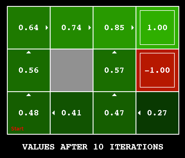
There are two absorb state, where the agent will get positive and negative rewards separately. As the Fig. above shows, VI always selects the action in the current iterations that enables the agent get much more rewards. The cell $3\times2$ is much nearer to terminal state $3\times4$ than start state $3\times1$, but after learning we still found that it’s better from state $3\times2$ to $3\times1$, then go along the direction arrows show to the terminal state.

Either PI and VI has the character in common that they assume the dynamic of the current environment is available. It means i.e. in the grid world the transition probability from each state to its successor state is given. In real word sometimes it’s either expensive to get this dynamics or it’s impossible to get those things. In the following section the samples-based algorithm will be represented.