Sample-based Method
Aside
In contrast to Model-based Methods such as PI and VI , in this part the Model Free Methods will be considered. For some case we don’t know the dynamics of our environment. It’s better we just interact with the environment to find the control policy.
Monte Carlo Method
Monte Carlo Method (MC) is a sample-oriented approach. It does not ask for the dynamic directly, it requires only experience, stimulated sequences of states, actions and rewards or it just interacts with the environment in a on-line way. Therefore it solves the RL tasks based on averaging sample returns. Concretely to say, the all state value in a sampling sequence will be updated equally. What if the sample distribution is not good, the policy we be more than we anticipate. For MC method we always need big amount of training data.
Temporal-Difference Learning
Temporal-Difference Learning (TD-Learning) is a combination of MC-method and dynamic programming (DP). One side it can use the stimulated experience to learn and at the another side it updates estimates based on the part already learned. What’s the temporal difference? Roughly speaking, it’s the state value or state action value between states. The simply TD method has the following form:
If we apply this TD method to action values, we get SARSA method, which uses only the five tuples . That’s why it’s called SARSA.
Q-Learning is another kind of TD-Learning. It approximates the optimal directly by learning the action value function independent the policy being followed. So it’s an off-policy TD control approach. As we said, the most amazing part or TD is it benefits one side from MC-method, it also bootstrap itself by considering the past experiences. Therefore there are two sides should be considered accordingly, the exploration and the exploitation. Exploration focus much more on to explore the unknown states, whereas exploitation thinks much heavily about using the current estimates greedily. For exploration we have i.g. greedy policy. With given exploration probability we select some action in current state randomly and with we just follow the current policy. In an non-deterministic MDPs play the noise a critical role. Noise means how uncertain than the agent gets a successor state after taking an action in current state. When the noise is quite big in your environment, it’d be quite if you use a better exploration policy.
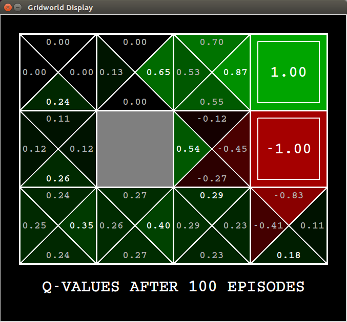
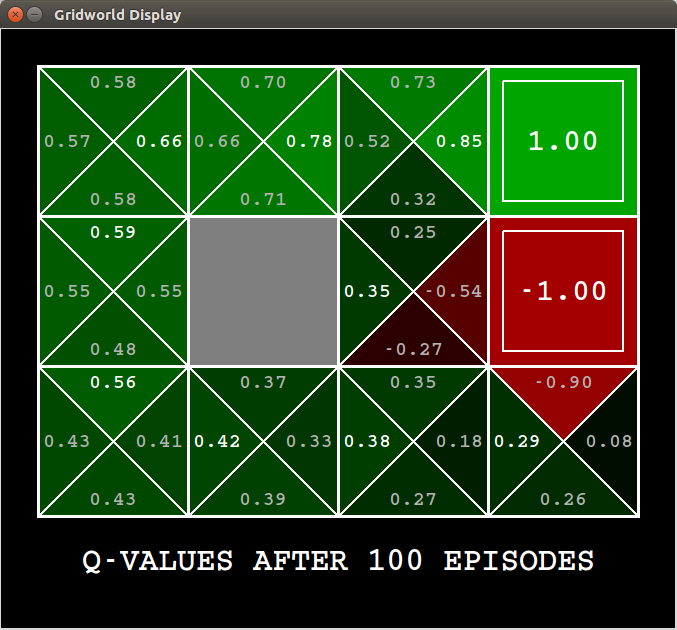
Here we have two diagrams: the topmost shows the value function without greedy policy and the botton one shows the value function with greedy policy with . As it shows, the action value of states are totally different after 100 iterations. Without random policy there are bunch of actions in states that are still undiscovered yet, whose action value are noted as $0.0$.
With exploration the Q-learning enables us to using the interaction with environment to stretch the optimal policy. But there are still polish points can be found in Q-learning. The Q-learner always back propagates the value state information or shortest path information from current state to the state where it comes from, as depicted as Fig.:
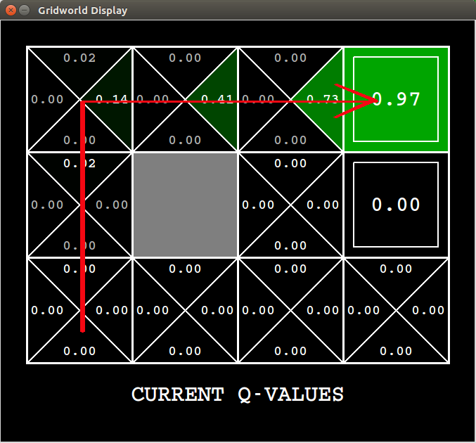
Actually we know from which states we get the current state implictly, so we can use this information to make Q-learning much effective? In next section we will find an answer for it.