Function Approximation

08 Jun 2017

Function Approximation

As in Sample-based Methods showed, the Q-learning can be used to learn a policy in a grid (or finite) world. It can also be ued in computer games or even some complicated task i.g. robotic navigation etc. What we met as so far is just the limit state space problem. For iterative updating it still needs much resource for calculating and for storing the state-action information. What if we have a continuous problem, then your table for DP updating will be exploded expanded. In pacman we used some features to learn the weight of each state action pair. These features are game based properties. Says how many pills you have or how far away you stand from ghost etc. If the feature has a very tiny change, but it will still be considered as different state as used before. Can we abstract this slightly changed information and handle them as maybe same states? With function approximation we’ll find a solution.

Feature Representation

Features are some sort of abstract of states in reinforcement learning tasks. It’s quite critical that how you extract features. If you create the feature in a very good way, the approximation results will be very explainable. There are various kinds of feature representing approaches. The most simple one is look-up table method. This method generates the feature for all states equally to one. As its simplicity it has presents a very poor representative ability for approximation. Another choice for generating feature is called tile-coding. Assume the state space spreads in a two dimensional space. The receptive field of features are grouped into partitions in this input space. Each partition is called tiling, here the big retangles as depicted in Fig.

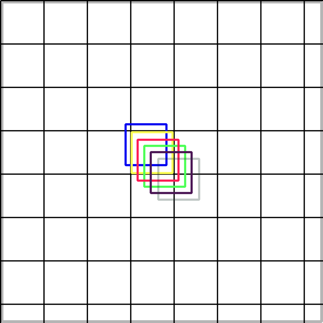
Feature generation by using teil-coding

Here we used six tilings. Each small cell is noted as tile. The size of cell implies the resolution of final approximation. As the tiling moves up and down, each cell will covered by the tilings. The different indexes of each tiling is then combined as feature vector. This approach is easy to implement and good at continuous tasks. For instance in the mountain-car problem, the car’s position and velocity can be represented in this state space. So we just move the tilings for getting the approximated features. There are also some coding-based approaches such as coarse coding or Kanerva coding and RBF. Those I’ve not used yet. Here I used the hand-crafted features that depends on the game itself very tightly. The representative ability of features depends on how many aspects you are going to take into account. This is really problem oriented features. Pacman game looks like in following Fig.

Pacman snapshot

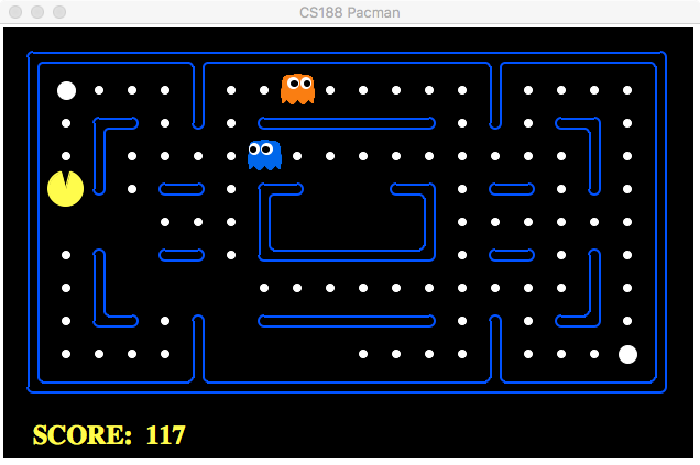
The rules are quite simple in pacman game: you should control the pacman to collect pills as much as you can to get a higher score and avoide your pacman from hunting by the ghosts. There are at least one ghost which try to hunt you. There are also some power pills that enable you to eat the ghosts. What you need to do is running for points and avoiding from ghosts.

Linear Function Approximation

In function approximation schema we don’t use the state directly, instead we use the feature-based state representation information, so the states can be represented as feature vectors. Each element of this vector represents a special feature in game state, such as the distance to ghost, number of ghost etc. Under this settings we can rewrite our action value function as:

$\begin{align} Q(s,a) &= w_1 f_1(s,a) + w_2 f_2(s,a) +\dots + w_n f_n(s,a)\\ &= \sum_{i=1}^{n} w_i f_i(s,a) \end{align}$

and the state value as: $\begin{equation} v(s) = \sum_{i=1}^{n} w_i f_i(s) \end{equation}$

In the normal Q-learning the action value in state $s$ with action $a$ updated as $Q(s,a) \leftarrow Q(s,a) + \alpha \times \delta$ ,where $\delta$ the temporal different defined as

$\begin{equation}\delta = \left[r + \gamma \max_a^\prime Q(s^\prime, a^\prime) \right] - Q(s,a)\end{equation}$ .

In the linear $Q$ -function the update step of $Q(s,a)$ is considered as updating the corresponding weight

$\begin{equation}w_i \leftarrow w_i + \alpha \times \delta \times f_i(s,a)\end{equation}$ .

This problem is actually a Linear Regression problem: we have the target value defined as

$\begin{equation}Q(s,a) = \left[r + \gamma \max_a^\prime Q(s^\prime, a^\prime) \right]\end{equation}$

and the estimated value

$\begin{equation}\tilde{Q}(s,a) = \sum_{k}w_k f_k(s,a)\end{equation}$ .

The total error can be defined as

$\begin{equation} \Delta = \sum_{i}\left(q_i - \tilde{q_i}\right)^2 = \sum_{i}\left(q_i - \sum_{k}w_k f_k(s,a)\right)^2. \end{equation}$

So the error will be minimized by gradient descent:

$\begin{align} \nabla_{w_m} \Delta &= \nabla_{w_m} \frac{1}{2}\left(q - \sum_{k}w_k f_k(s,a) \right)^2\\ &= -\left(q_i - \sum_{k} w_k f_k(s,a)\right) f_m(s,a)\\ &= w_m + \alpha \left(q_i - \sum_{k} w_k f_k(s,a)\right) f_m(s,a). \end{align}$

In pacman the features as we said can be the distance from agent to ghost, or the number of power pills, or the panic time of ghost etc. Here we used there relative features: the distance to pill, the distance to ghost and a bias. After 1000 iterations training, it got the 98 $\%$ times to win the game. Linear function approximation works quit well in this case. What if we have much more complicated features that have high dimensions. It’s not a good choice to optimize this problem by yourself. There are many solvers can be used for optimizing problems.In next section the convex optimization solver CVX will be introduced.

Approximate Linear Programming

CVX is a modeling system for constructing and solving disciplined programs such as linear and quadratic programs, second-order cone programs. The usage of CVX is very user-friendly. What need to be at first initialized by you is to form your problem into a convex problem. Convex problem means the problem involved can be optimized (minimized) over a convex sets, further information see in section Optimization. CVX can be integrated either in Matlab or Python. In the following code pieces we used CVX to solving the linear equation $\mathbf{Ax=b}$ .

% declare variable 
m = 20; n = 10;
A = randn(m,n); b = randn(m, 1);

% using CVX
cvx_begin
  % define a affine variable in CVX
  variable x2(n)
		    
  % minimize the euclidean distance
  minimize( norm( A * x2 - b, 2) )
cvx_end

With keyword $cvx\_begin$ the cvx body begins, in its body all the necessary variables will be declared by using $variable$ keyword. After declaring we you intend to do then with $cvx\_end$ close the syntax definition. This procedure will be automatically invoked by Matlab or Python.

Let’s go back to our VI and see how it’ll be solved by CVX. In VI we solve the Bellman equation in the following way:

$\begin{equation} V(s)= \max_a \sum_{s^\prime}p(s^\prime|s,a) \left[ r(s, a, s^\prime) + \gamma V(s^\prime) \right], \text{for } \forall s. \end{equation}$

This equality (or $\max$ operator ) is nonlinear, so we can relax this problem by introducing constrains. If we have a look at the Eq. above, it’s actually the equivalent to:

$\begin{equation} V(s) \ge \sum_{s^\prime}p(s^\prime|s,a) \left[ r(s, a, s^\prime) + \gamma V(s^\prime) \right], \text{for } \forall s,a. \end{equation}$

Hence we can solve VI by solving

$\begin{equation} \min d^T V s.t. \forall s, a: V(s)\ge \sum_{s^\prime}p(s^\prime|s,a) \left[ r(s, a, s^\prime) + \gamma V(s^\prime) \right], \end{equation}$

where $d$ is a arbitrary vector. This is the relaxing process. Let $T$ stands for the Bellman operator, this VI equation can be simplified as

$\begin{equation} \min d^T V s.t. V \ge TV, \end{equation}$

For a feasible solution of this constrained optimization, we have $V \ge TV$ . Bellman operator itself is monotonic operator, it means $V_1 \ge V_2 \implies TV_1 \ge TV_2$ . So it works also out for the optimal policy:

$\begin{equation} TV \ge T(TV) \ge T(T(TV)) = T^3 V \dots \implies V \ge TV \ge T^2 V \ge \dots \ge TV = V_\star. \end{equation}$

This equality means after iterations the feasible regions of relaxed VI is compacted repeatedly and we’ll then get the optimal policy this way. So we can find $V_\star$ by solving the following linear program:

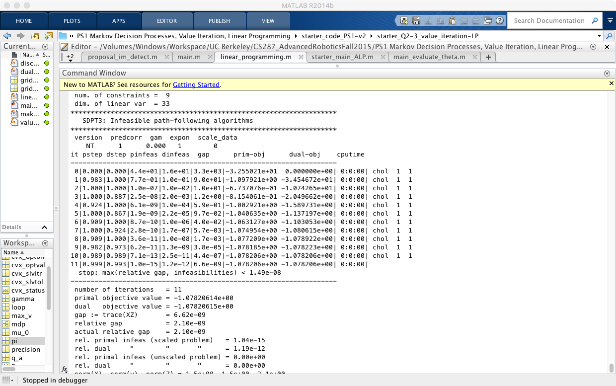
$\begin{equation} \min_V d^T V \ s.t. V \ge TV, \end{equation}$

We used CVX to solve this equation, the result is the same as we did in Model-based Methods. Below shows the outputs of CVX after successfully sovled our value iteration problem:

The result of CVX for solving VI

Let’s continuously go along this way straight to find the approximate linear programming. In linear function approximation settings the state value is represented by a linear combination of its features and the weight of features correspondingly. As it changes, so the VI function has been also changed accordingly: $\begin{equation} \min_{V,r} {d}^T {\phi} {r} \ s.t. {\phi r} \ge T ({\phi r}), \ V = {\phi r} \end{equation}$ After all substitutions we got this optimization problem:

$\begin{equation} \begin{split} \min_r \sum_{s\in S}d(s) \sum_{i}\phi_i(s) r_i \\ s.t. \forall s \in S, a: \\ \end{split} \end{equation}$ $\begin{equation} \sum_{i}\phi_i(s) r_i \ge \sum_{s^\prime} p(s^\prime|s, a)\left[ r(s, a,s^\prime) + \gamma \sum_{j} \phi_j(s^\prime) r_j \right] \end{equation}$

That’s the basic idea of finding a optimal policy in a finite state problem by using approximate linear programming. It works sometime astonishing good and sometiem quite in opposite. The feature extract plays a critical role.

Reinforcement Learning