Recurrent Neural Network
Basic
In contrast with densely connected neural network or Convolution Neural Network, the recurrent neural network delivers a big variety in deep learning model. Let’s have a essential picture of this model at first. RNN is a kind of State-Space Model that has the following structure
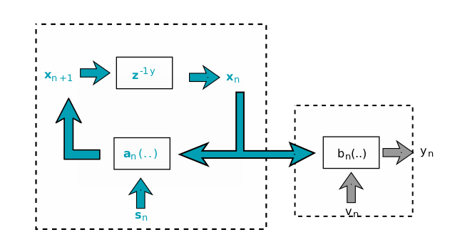
The left part of this diagram is the system model, where is a vectorial function, is the current value of state, denotes the value of subsequent state, is a time delay unit and is the dynamic noise. has the following definition form: \begin{equation} x_{n+1} = a_n(x_n, s_n) \end{equation} The right part is the measurement model in this state space system, where the noise in measure and the observable output that defined as \begin{equation} y_n = b_n(x_n, v_n) \end{equation} The evolution process varies over time is depicted as follows:

As we can see that the structure of this model takes the time steps into account. Actually this is the Bayesian Filtering system. Our RNN has also the similar structure, whose evolution structure over time depicted as given by:
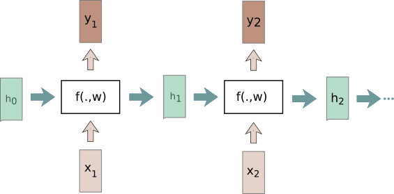
This structure depicts a interesting characters: the generated hidden state in previous state is fed in the subsequent state . The weight connecting the input and hidden state are reused in each time step , at each time step there will be a output generated. Formally this can be defined as follows:
When this model works over time steps, the context information (or prior information) in hidden neurons will be stored and passed in the next time step so that learning task that extends over a time period can be performed.
Image Captioning
As a brief introduction of the RNN’s structure was given. Here is an example that uses this model to caption a image. Image captioning means, say, you give a image to a model. This model learns the saliencies firstly. After running our model with this saliencies you’ll get a consice description about what’s going on in this given image. For image captioning we need extra information that represents the image to be captioned. This information can be learned by other learning model, i.e. convolution neural network. The captioning vocabulary consists of string library, but for simplifying the learning process this vocabulary is converted in to integers that can be easily handled as vectors. At the test time we get a bunch of integers as return results, then we decode it into the original word string correspondingly.
Training Stage
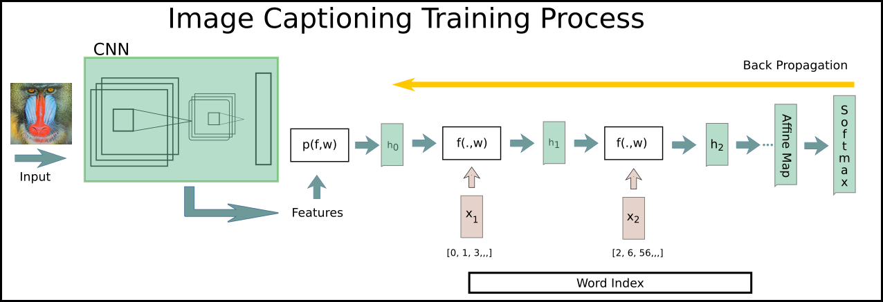
At training time features of images are trained at first by convolution network. These features are projected with this affine function to initial hidden state of our network. The vocabulary indexes are coded in a word embedding layer that maps the word to matrix that we can perform our for- and -backward propagation numerically. The training caption data consists of a image looks like as follows:
Training Stage
Each caption is tagged with some extra information likes and tokens. All the captions vocabularies are handled as matrix, cause we can’t use them directly, say for instance, in forward propagation flow. During the training the weight of corresponding words will be updated, which also reflects the distribution of vocabularies. Also at each time step the last hidden state is used to forward propagate the “context information” over time steps. This context information implies the potential connections in original training data. The word score corresponding to features are calculated in a affine layer and fed into softmax layer to calculate the loss function. The yellow arrow indicates the direction of back propagation. The whole training task is actually not so complicated. The normal update rules can also be used for updating the parameters here. The back progapation works symetrically as we do in normal case.
Test Stage
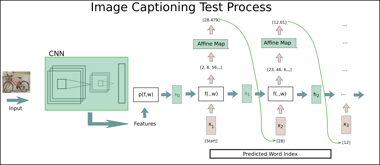
The test process is shown in the figure below. The feature conversion is just same as we did in training process. Now the input to our model is little different. At the beginning of test the first word feed to model is token. The feature will be used in and combined with the hidden state. The rest stays same as in training state excpet the last step, at which we will get a word that has the maximal score. The word with maximal score is stored in captions vectors and used in subsequent iterations. After iterations the caption vectors will be returned and decoded in corresponding text. The procedure repeats over all the features. The output is just then a couple of words that we got in each time step.
Pros vs. Cons
The workflow of this model in the area of image caption has been briefly presented. The hidden state are always newly generated as training. So as the error propagates backwards, this should be summed in total time steps but initial hidden state. The content information in previous neurons has been stored and forwards propagated via hidden state and the relation between features and words over vocabulary is mapped in the the affine layer and the corresponding importance is reflected in the vocabulary weights in this layer. Here the vocabulary is also important, or in other words the distribution of words in vocabulary is very essential to caption images. If the words are not good selected enough, the caption will be meanless of human.
The structure of this model is quite simple to understand. Each hidden state just stacked over time steps that lurks the potential problem. Let’s recap our training process again. We feed our features as inputs to RNN, and combined the non-linearity, infinitesimal changes to update our parameters over time distance. This may do not effect the training or be neglectable. Or if we have a big change in inputs that are unfortunately not measured by the gradient as time changes. This so-called Vanishing-gradients problem downgrades the learning that has long-term dependencies in gradient-based models.For solving this problem we can use non-linear sequential sequence state model like Long Short Term Memory